ElectronView Electroluminescence Quantum Efficiency Measurement Software Tutorial

Overview

ElectronView is professional measurement software developed by Pynect for the PYN-E560 series external quantum efficiency (EQE) measurement system. It integrates core functions such as radiometric calibration, EQE measurement and LED lifetime testing, supports automatic control of Keithley 2400/2450 series source meters and the probe station, and can complete the full measurement workflow from voltage sweep to EQE calculation in one click. Based on the PYN-E560 measurement system, this article details the complete operating procedures for software installation, radiometric calibration, EQE measurement and lifetime testing.

---

1. Radiometric Calibration

1.1 Why Radiometric Calibration Is Needed

In EQE measurement, the relative spectral distribution acquired by the spectrometer must be converted into an absolute optical power distribution before physical quantities such as luminance, radiance and photon count can be calculated, and EQE obtained. Due to differences in grating efficiency, detector quantum efficiency, fiber transmittance and other factors, different spectrometers produce different relative spectral distribution curves. The purpose of radiometric calibration is to convert the relative spectral distribution into an absolute optical power distribution. After radiometric calibration, the optical power distributions measured by different spectrometers will be consistent.

1.2 Entering the Radiometric Calibration Interface

After opening ElectronView, follow these steps to enter the radiometric calibration interface:

1. Click Instrument Parameters in the lower-left corner (Figure 1, marker 1)
2. Click Radiometric Calibration in the top menu bar (Figure 1, marker 3)
3. Click the Start button on the left side of the top menu bar to make the spectrometer read the spectrum in real time

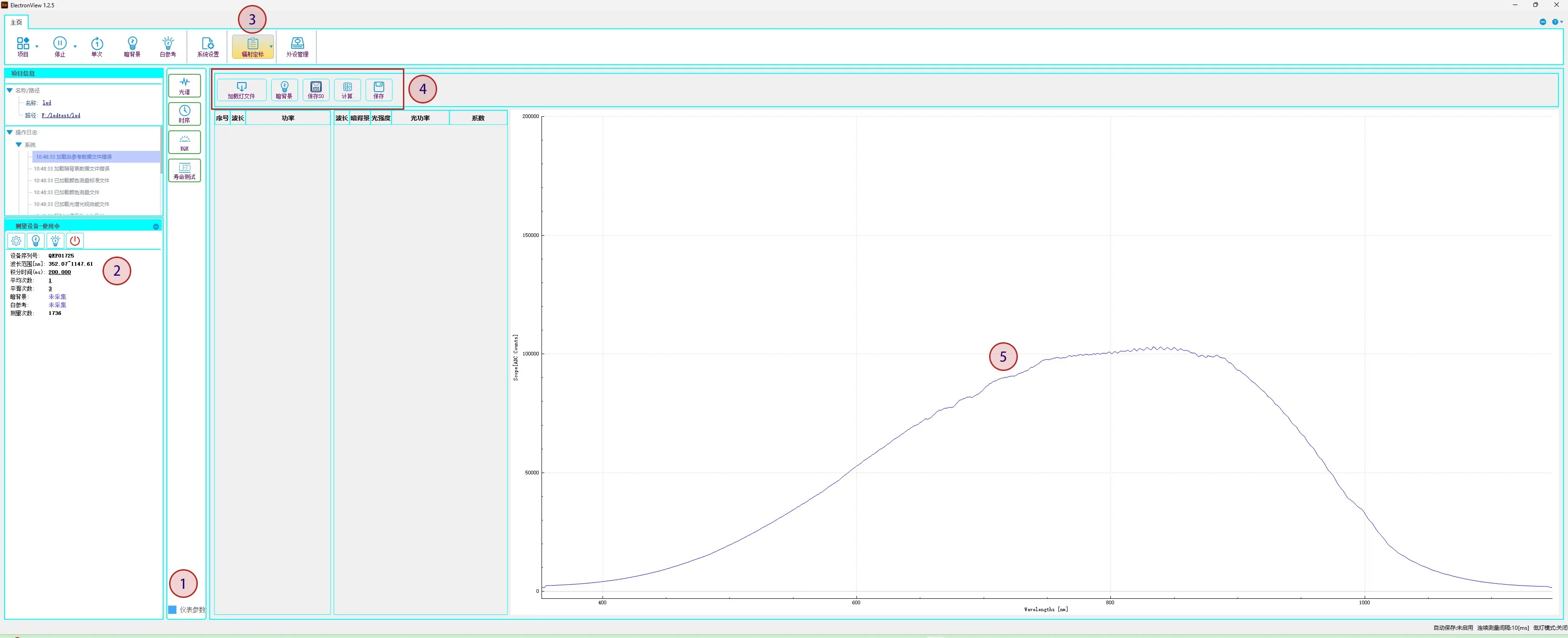
Figure 1: Radiometric calibration software interface

1.3 Radiometric Calibration Procedure

Step 1: Fit the radiometric calibration cover

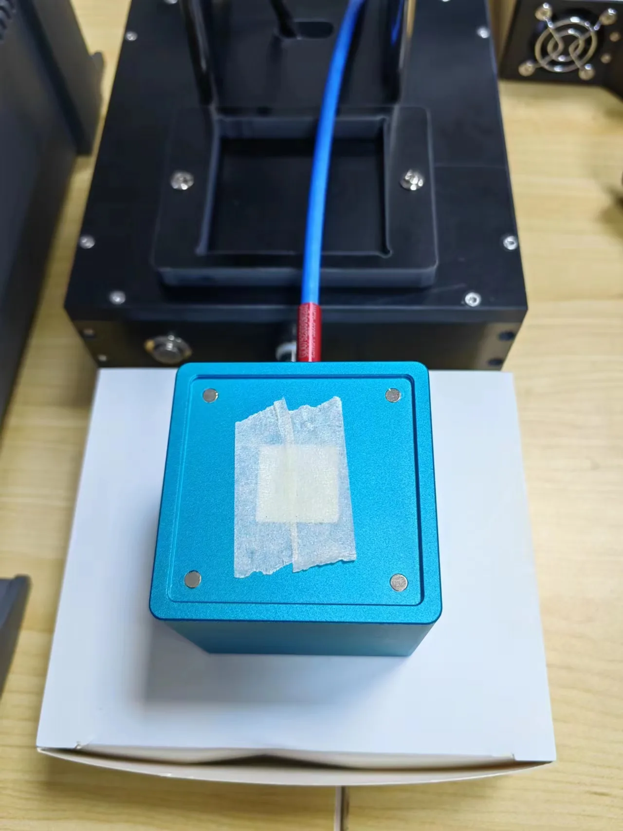
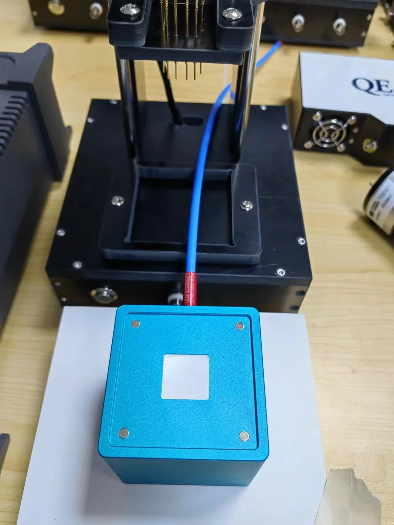
On first use, if the integrating sphere sample port has a sealing sticker, peel it off first (Figure 2, left), then fit the radiometric calibration cover (Figure 2, right, and Figure 3). It is recommended to take the integrating sphere out of the probe station's fixing slot and raise it with a paper box or similar to avoid pulling on the fiber.

Peel off the sealing sticker	Fit the radiometric calibration cover

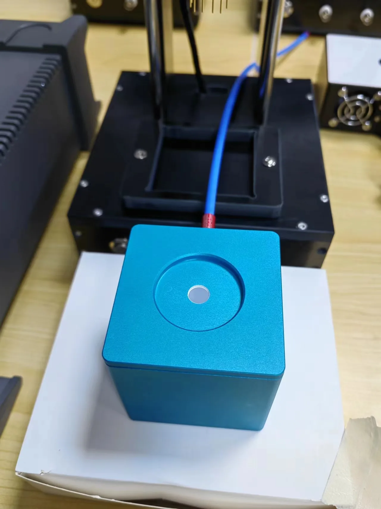Figure 2-3: Fitting the radiometric calibration cover

Step 2: Warm up the light source and place it

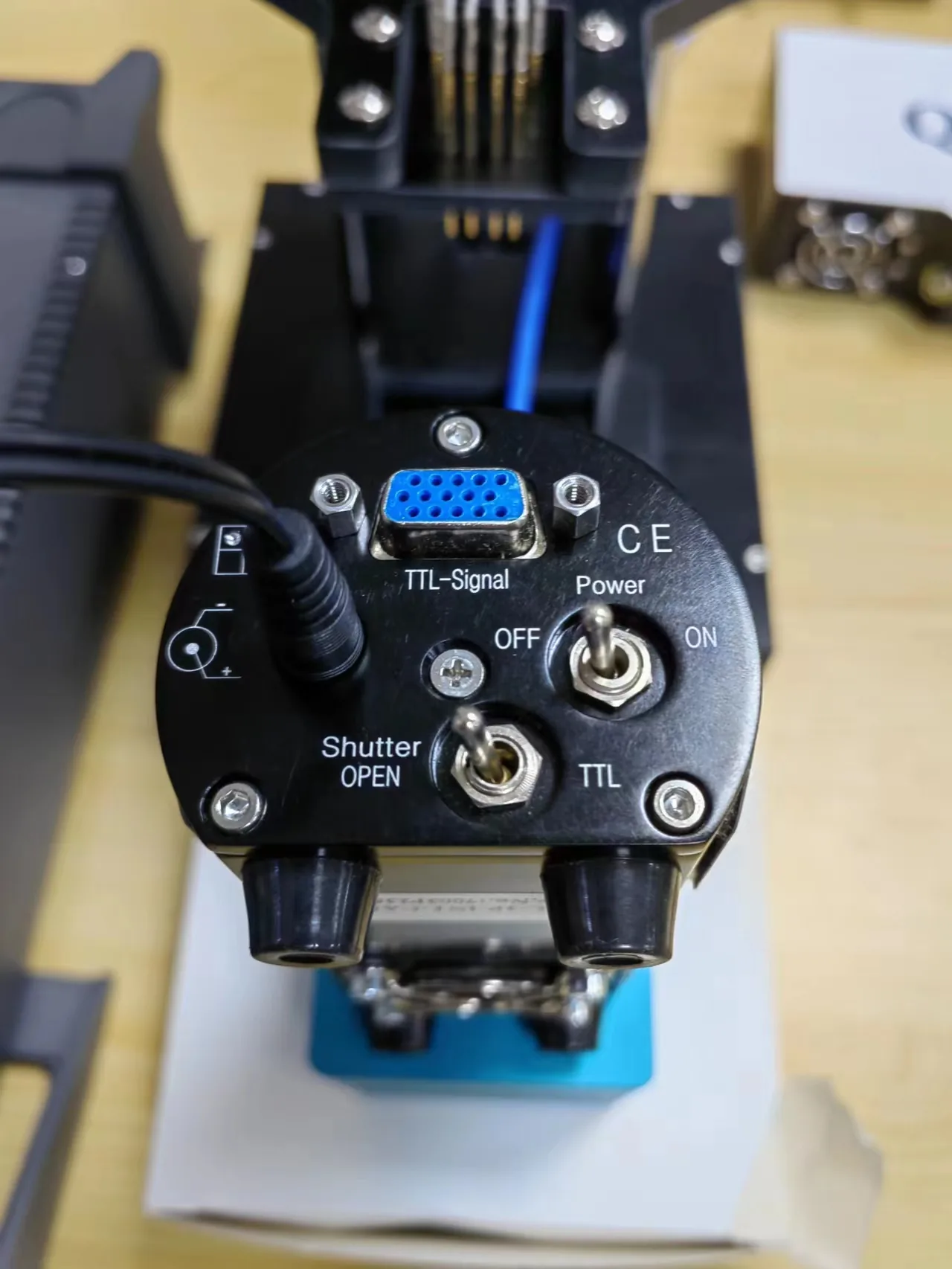
1. Turn the Power switch of the radiometric calibration source to ON (Figure 4, left) to switch it on
2. Warm up for 5 minutes until the source output is stable
3. Place the radiometric calibration source on the radiometric calibration cover (Figure 4, right)

Switch on the light source	Place it on the cover

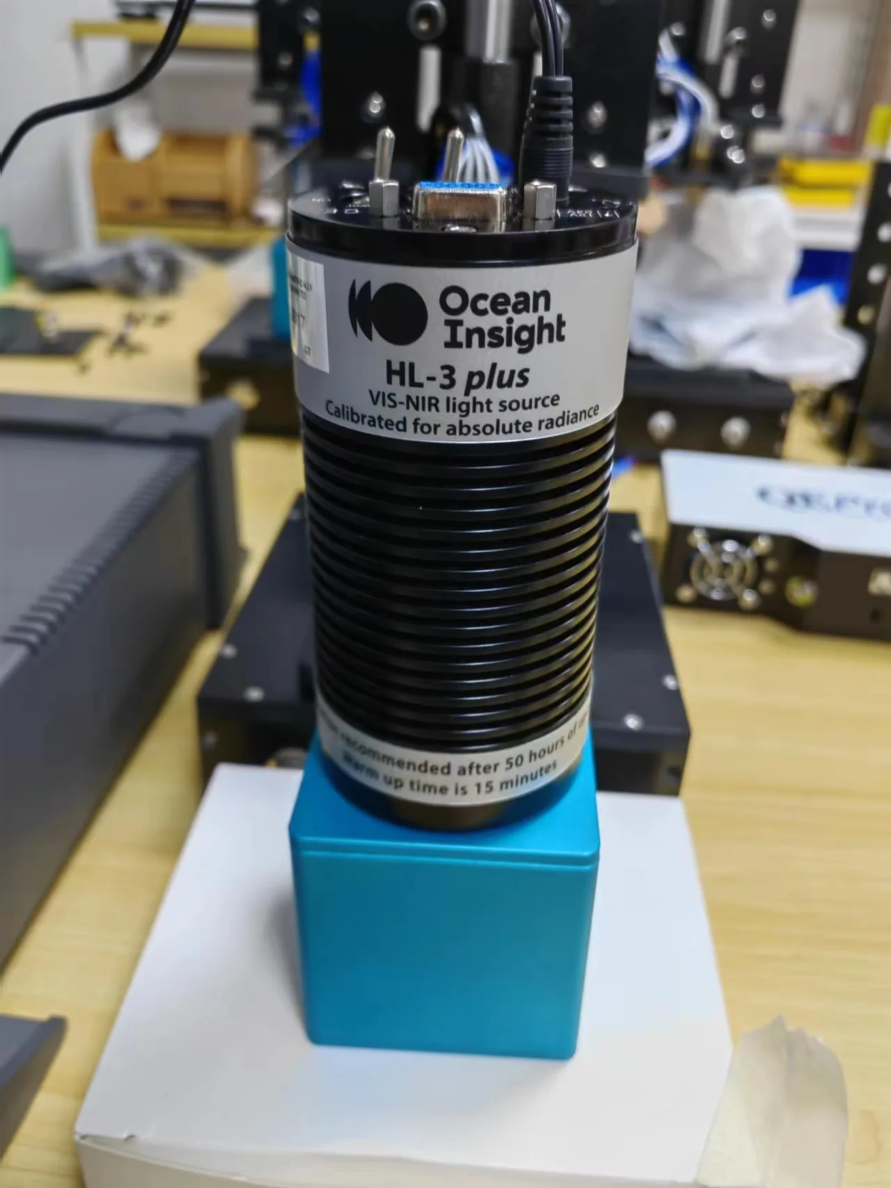Figure 4: Radiometric calibration light source

Step 3: Set the spectrometer measurement parameters

Adjust the spectrometer integration time so that the spectral intensity is around 100,000 counts (see Figure 1, marker 5 area). Then set an appropriate number of averages (1 is recommended) and smoothing passes (3 is recommended).

Step 4: Load the lamp file

Prepare the lamp file that comes with the radiometric calibration source (it must be converted to .txt format), click the Load Lamp File button, and select the prepared txt lamp file in the pop-up dialog.

Step 5: Store the dark background

Set the Shutter switch of the radiometric calibration source to the middle position so that the internal baffle blocks the light; the spectral curve should now be almost zero. Click the Dark Background button to store it.

Step 6: Store the relative spectrum of the radiometric calibration source

Set the Shutter switch to the left OPEN position; the spectral curve should now be visible. Click the Save S0 button to read the current relative spectrum (with the dark background already subtracted).

Step 7: Calculate and save

Click the Calculate button and the software automatically computes the radiometric calibration coefficients (usually within 3 seconds). A corresponding message appears in the upper-left corner when the calculation finishes. Click the Save button and the calibration coefficients are saved to the config file in the software installation directory.

Tip: The next time the software is opened, the radiometric calibration coefficient file is loaded automatically, so recalibration is not required. However, if the optical path has been disassembled (e.g. the integrating sphere or fiber was replaced), recalibration is required.

---

2. EQE Measurement

2.1 Connect Peripherals

After entering the software, the spectrometer connects automatically. The source meter and probe station must be connected manually:

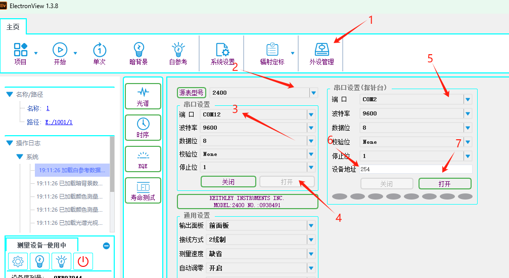
1. Click Peripheral Management to open the source meter and probe station settings interface
2. Select the source meter model (e.g. Keithley 2400 / 2450)
3. Select the number — for RS232 source meters, select the corresponding serial port number; for USB source meters, the device number is displayed automatically
4. Click Open Source Meter; the source meter model and serial number are displayed when successful
5. Select the serial port number corresponding to the probe station
6. Leave the device address at the default of 254
7. Click Open Probe Station

2.2 EQE Measurement Interface

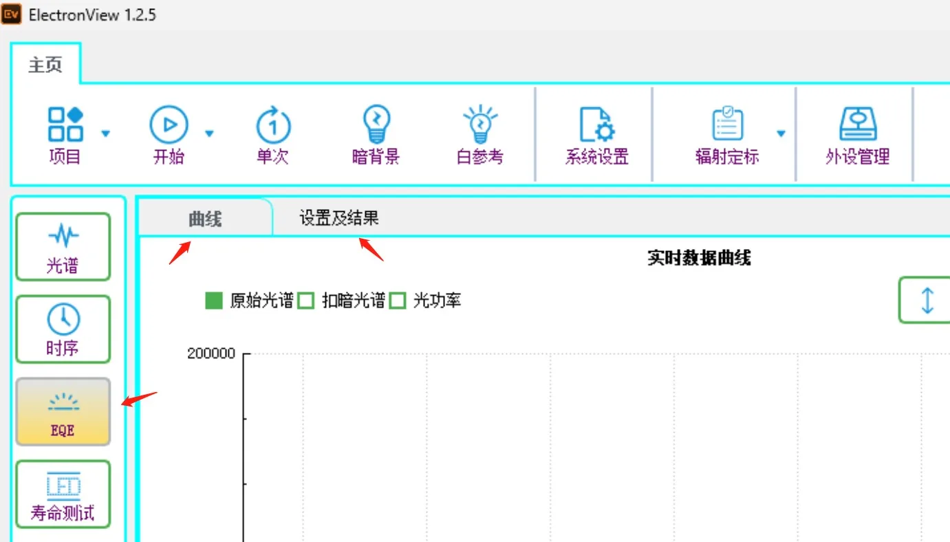
Click the EQE application function on the left to enter the EQE measurement interface. You can switch between the Curve and Settings & Results tabs.

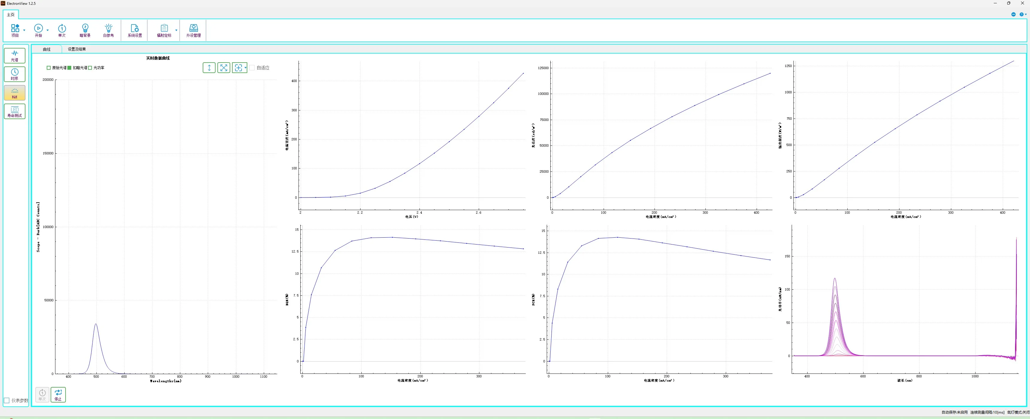
Figure 5: EQE measurement interface

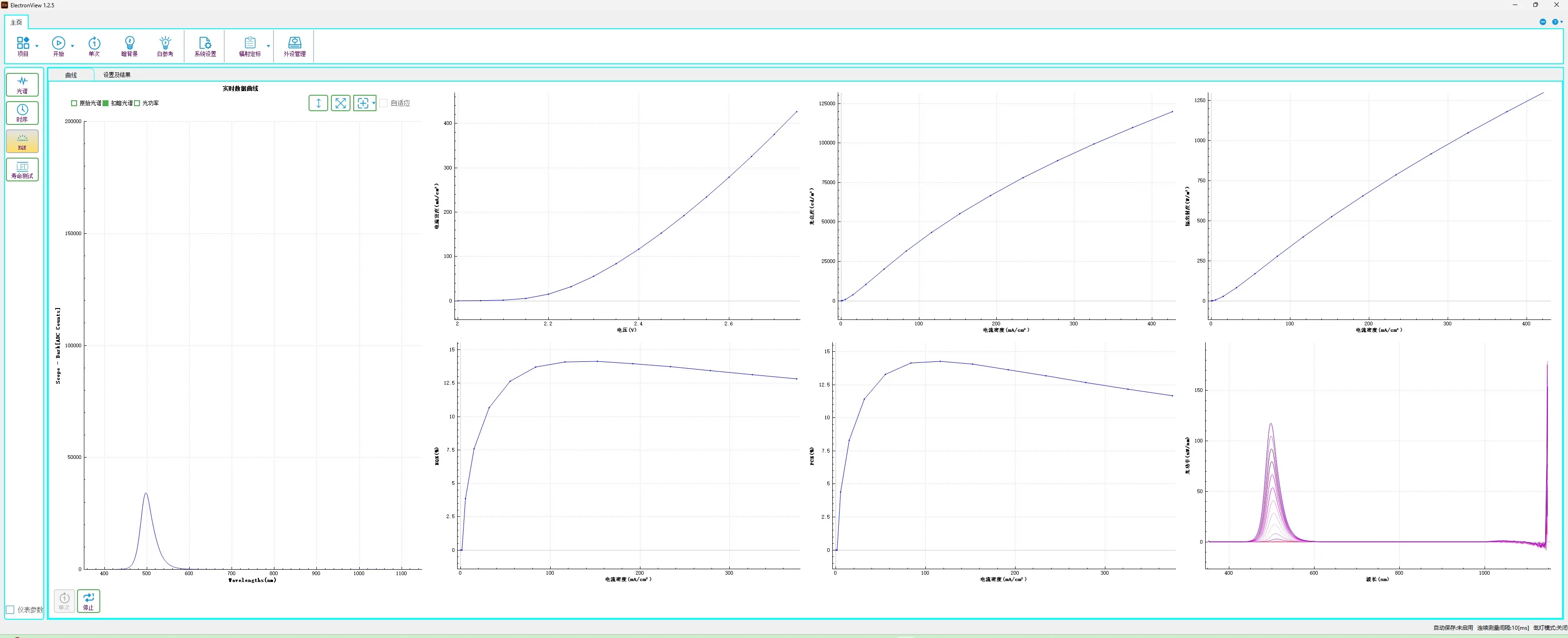
The curve interface displays the following four curves in real time:
- Real-time data curve: the spectrometer's raw spectrum or optical power (switchable in the upper-left corner)
- Current density vs. voltage curve: reads the source meter's voltage and current in real time; current density = current ÷ LED emission area
- Luminance vs. current density: luminance corresponds to the 380-780 nm visible band
- Radiant exitance vs. current density: radiant exitance = optical power ÷ emission area

2.3 Set Measurement Parameters

Switch to the Settings & Results tab and fill in the following parameters:

Left parameter settings	Right parameter details

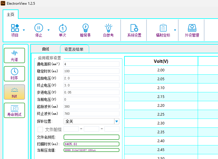Figure 6: EQE test parameter settings

Parameter	Description
Energized area	LED emission area, i.e. the overlapping area of the cathode and anode
Settling time	Time required for the source meter output to stabilize; 100 ms by default is sufficient for the 2400/2450
Start voltage	Start voltage supplied by the source meter
Stop voltage	Cut-off voltage supplied by the source meter
Step voltage	Voltage interval for each source meter supply step
Start wavelength	Start wavelength for calculating luminance and photon count, 380 nm by default
Stop wavelength	Cut-off wavelength for calculating luminance and photon count, 780 nm by default
Probe position	Number of the LED under test; only one LED can be lit at a time

2.4 Place the Sample

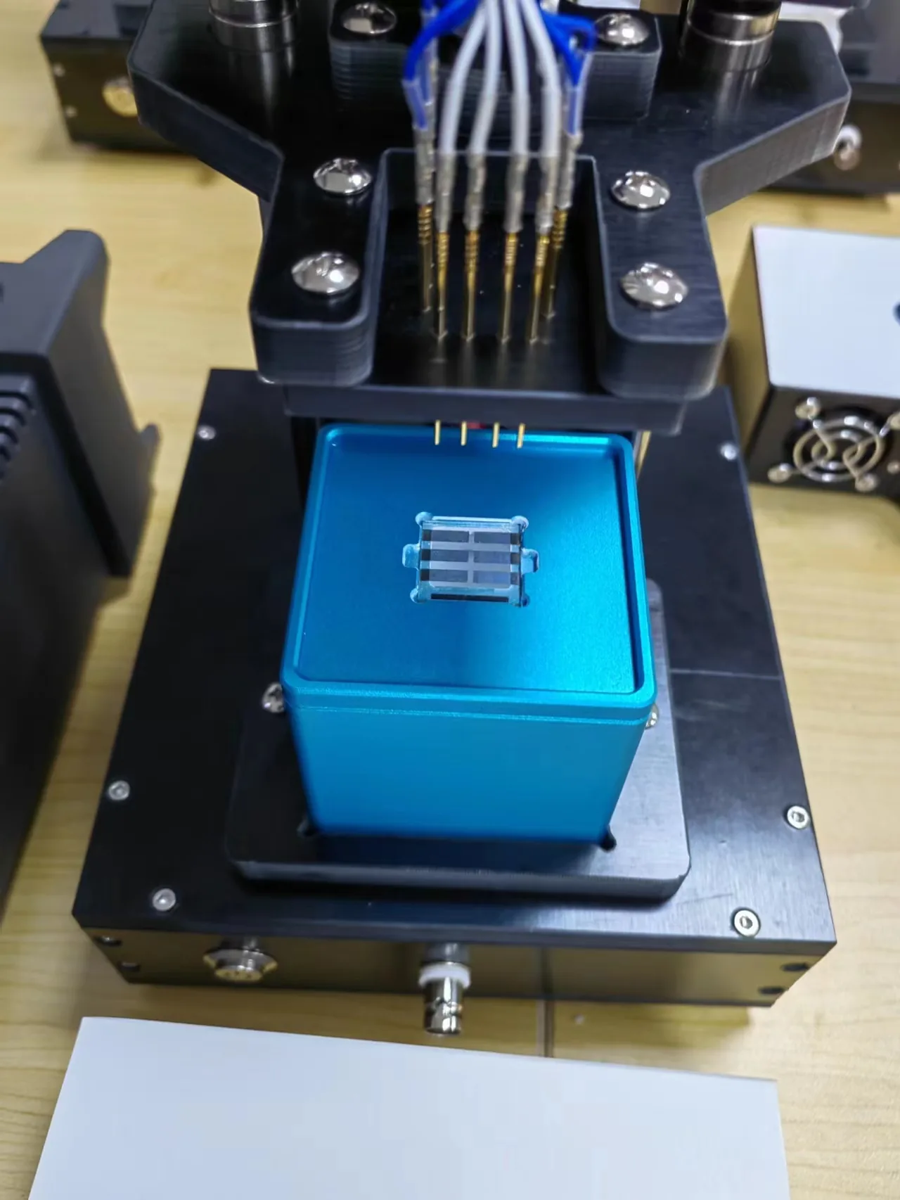
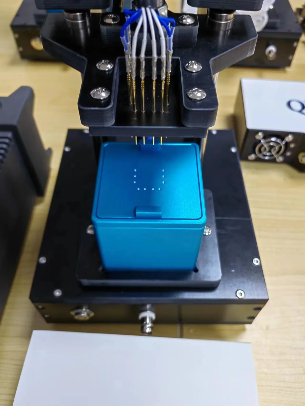
Sample-slot cover	Place the LED sample	Press down the handle

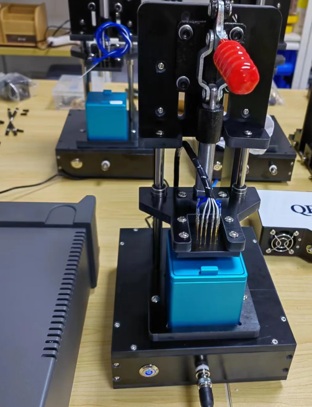Figure 7: Placing the LED sample

Placement procedure: remove the sample-slot cover → place the LED sample → put the sample cover back → press down the handle. The probe tip has some elasticity; good contact is achieved by the weight of the handle alone, with no need to keep pressing.

2.5 Start the Measurement

After setting the parameters, click the Continuous button in the lower-left corner, and the source meter increases the voltage step by step to test.

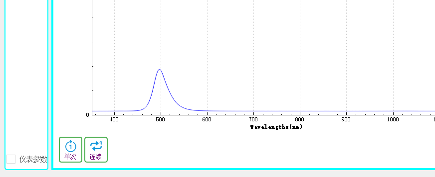
Figure 8: Single and continuous measurement

During the measurement you can switch tabs to view in real time:
- Curve tab: observe the changes of the four live curves
- Settings & Results tab: view the tabular data

EQE live measurement curves	EQE measurement table

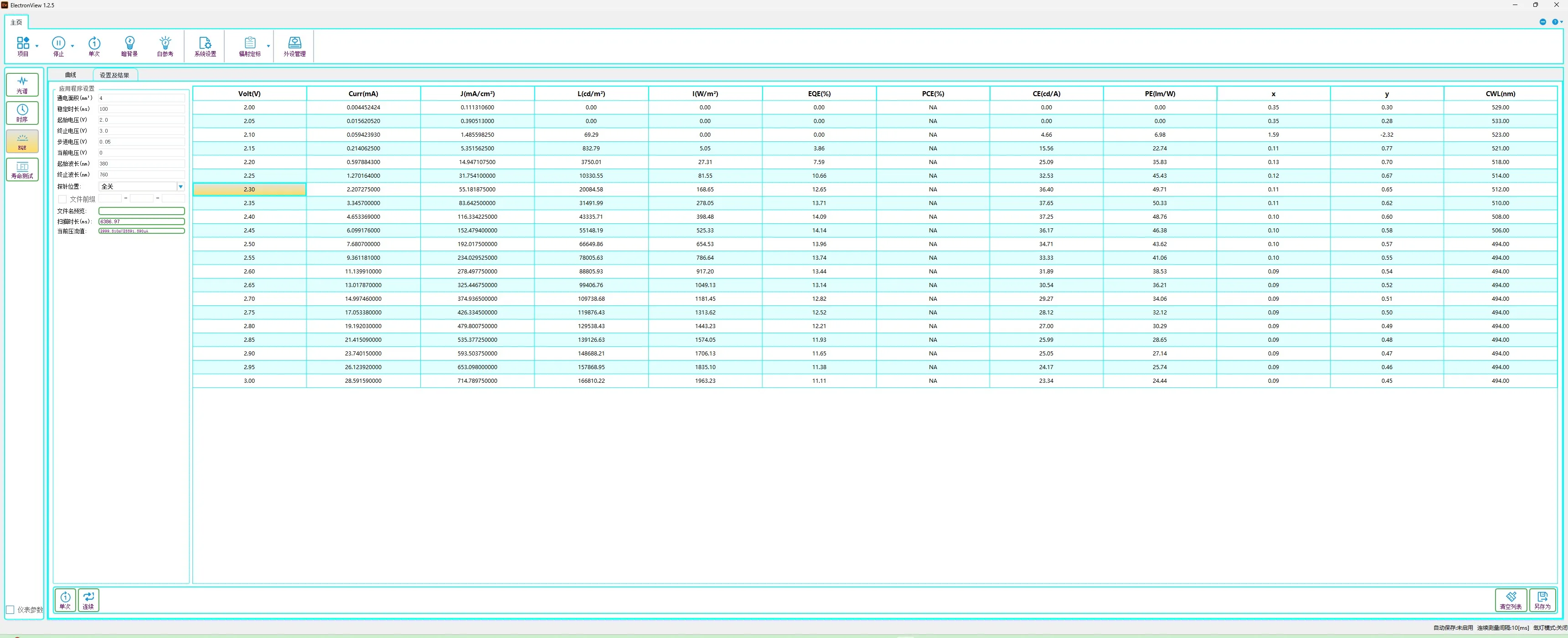Figure 9-10: EQE measurement process

2.6 Data Export

EQE table data

In the table interface, click the Save As button in the lower-right corner, enter a file name and export to the specified path.

EQE optical power data

In continuous measurement mode, the optical power distributions corresponding to each step-voltage increment are automatically saved to the data folder in the project path after the measurement completes, with file names in the format probe-number-time-Power.csv. The first column is wavelength, and the subsequent columns are the optical power data at the corresponding step voltages.

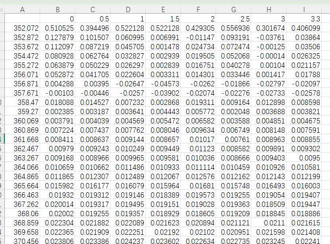
Figure 11: Optical power data at different voltages

---

3. LED Lifetime Testing

3.1 Set the Source Meter Output

Taking the most common constant-current test as an example:

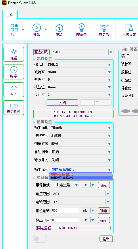
1. Select the Single-step constant current output mode

Select output mode	Set parameters

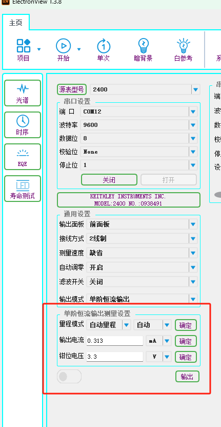2. Select the corresponding current range and set the current value

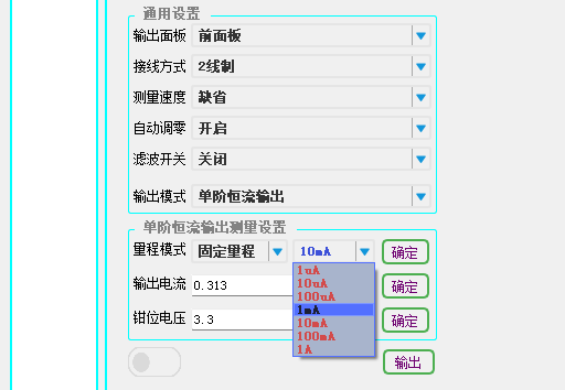
Note: The default is auto-range mode, but for higher current output accuracy it is recommended to manually select the corresponding current range. For example, if the current value is 0.313 mA, select the 1 mA range. After setting, click OK to apply.

3.2 Lifetime Measurement

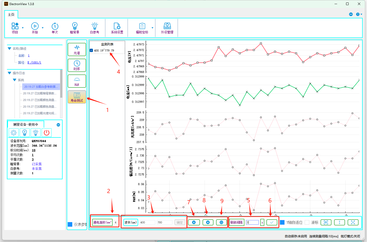
Operating steps:

1. Select the Lifetime Test function (marker 1)
2. Set the Energized area (marker 2) and Wavelength range (marker 3); after clicking OK, the closest spectral range is shown in the detection list (marker 4)
3. Set the measurement interval (marker 5), 1 s by default. Click OK (marker 6) to apply after setting
4. Click Start (marker 7) to begin automatic testing at the set interval
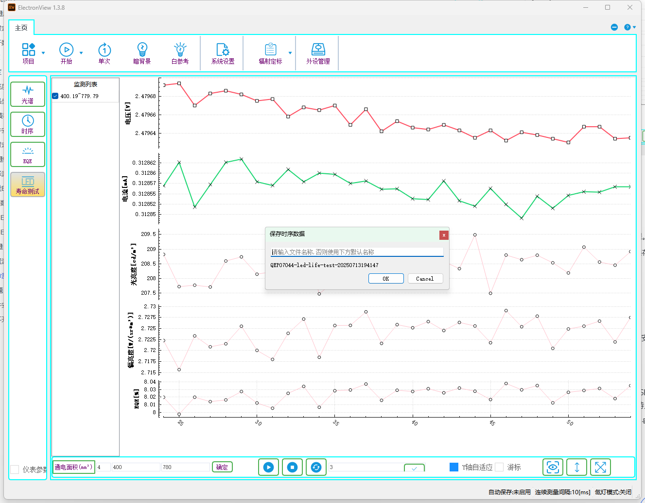
5. Click Stop (marker 8) to stop the measurement; a save dialog pops up

---

4. FAQ

4.1 Software Installation

For Windows 10 and above, it is recommended to install to the C drive in administrator mode, otherwise disk-permission restrictions may prevent the software from completing registration and cause problems.

4.2 Cannot Open the Source Meter

• Keithley 2450 (USB interface): in most cases the driver is not installed correctly. Contact the source meter manufacturer or Pynect technical support for remote assistance
• Keithley 2400 (RS232 serial port): mainly due to selecting the wrong serial port number; confirm the correct COM port number in Device Manager

---

This article was compiled by Pynect; images are from the PYN-E560 measurement system user manual.